Visualizing Labelled Graph States

This example visualizes GraphQOMB’s graph-state IR, including input/output registration and non-XY measurement planes.

import matplotlib.pyplot as plt
import numpy as np

from graphqomb.common import Axis, AxisMeasBasis, MeasBasis, Plane, PlannerMeasBasis, Sign
from graphqomb.graphstate import GraphState
from graphqomb.random_objects import generate_random_flow_graph
from graphqomb.visualizer import visualize

# Create a random flow graph
random_graph, flow = generate_random_flow_graph(5, 5)


# Visualize the flow graph
ax = visualize(random_graph)
plt.show()
print("Displayed flow graph")

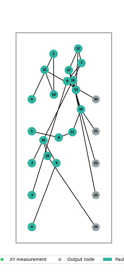
Displayed flow graph

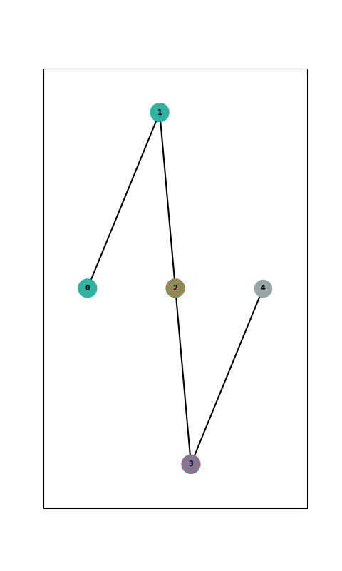
Create a demo graph with different measurement planes and input/output nodes

# Define graph structure with named nodes
nodes = ["input1", "input2", "internal1", "internal2", "internal3", "output1", "output2"]
edges = [
    ("input1", "internal1"),
    ("input2", "internal2"),
    ("internal1", "internal3"),
    ("internal2", "internal3"),
    ("internal3", "output1"),
    ("input1", "output2"),
]
inputs = ["input1", "input2"]
outputs = ["output1", "output2"]

# Define measurement bases for nodes
meas_bases: dict[str, MeasBasis] = {
    "input1": AxisMeasBasis(Axis.X, Sign.PLUS),
    "input2": PlannerMeasBasis(Plane.XY, np.pi / 6),
    "internal1": PlannerMeasBasis(Plane.XZ, np.pi / 4),  # XZ plane with angle π/4
    "internal2": PlannerMeasBasis(Plane.YZ, np.pi / 3),  # YZ plane with angle π/3
    "internal3": PlannerMeasBasis(Plane.XZ, np.pi / 2),  # XZ plane with angle π/2
}

# Create graph state from structure
demo_graph, node_map = GraphState.from_graph(
    nodes=nodes, edges=edges, inputs=inputs, outputs=outputs, meas_bases=meas_bases
)

print("Demo graph with XZ and YZ measurement planes:")
print(f"Input nodes: {list(demo_graph.input_node_indices.keys())}")
print(f"Output nodes: {list(demo_graph.output_node_indices.keys())}")
print(f"All physical nodes: {demo_graph.physical_nodes}")
print("Internal nodes with measurement bases:")
for node, basis in demo_graph.meas_bases.items():
    print(f"  Node {node}: {basis.plane.name} plane, angle={basis.angle:.3f}")

# Visualize the demo graph with labels
ax = visualize(demo_graph, show_node_labels=True)
plt.show()
print("Displayed demo graph with labels")

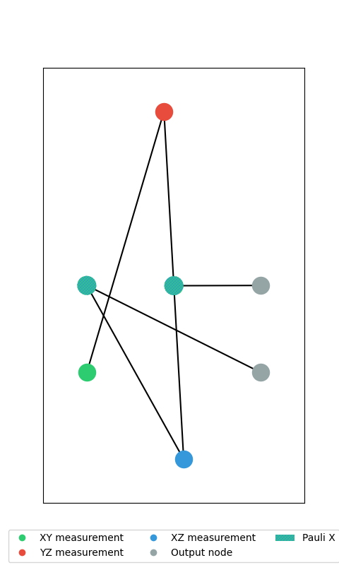
# Visualize without labels to see just the colored patterns
print("\n--- Same graph without node labels ---")
ax = visualize(demo_graph, show_node_labels=False)
plt.show()
print("Displayed demo graph without labels")

• 
• 

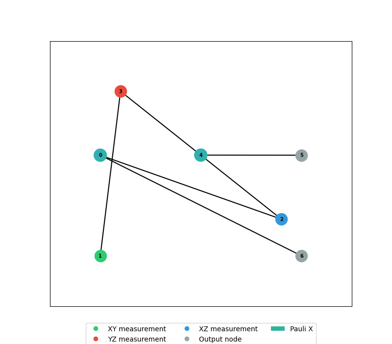
Demo graph with XZ and YZ measurement planes:
Input nodes: [0, 1]
Output nodes: [5, 6]
All physical nodes: {0, 1, 2, 3, 4, 5, 6}
Internal nodes with measurement bases:
  Node 0: XY plane, angle=0.000
  Node 1: XY plane, angle=0.524
  Node 2: XZ plane, angle=0.785
  Node 3: YZ plane, angle=1.047
  Node 4: XZ plane, angle=1.571
Displayed demo graph with labels

--- Same graph without node labels ---
Displayed demo graph without labels

Create another demo graph with Pauli measurements (θ=0, π) Define Pauli measurement graph structure

pauli_nodes = ["input", "x_meas", "y_meas", "z_meas", "output"]
pauli_edges = [
    ("input", "x_meas"),
    ("x_meas", "y_meas"),
    ("y_meas", "z_meas"),
    ("z_meas", "output"),
]
pauli_inputs = ["input"]
pauli_outputs = ["output"]

# Define Pauli measurement bases
pauli_meas_bases = {
    "input": AxisMeasBasis(Axis.X, Sign.PLUS),  # X+
    "x_meas": AxisMeasBasis(Axis.X, Sign.PLUS),  # X+: XY plane, θ=0
    "y_meas": AxisMeasBasis(Axis.Y, Sign.PLUS),  # Y+: YZ plane, θ=π/2
    "z_meas": AxisMeasBasis(Axis.Z, Sign.MINUS),  # Z-: XZ plane, θ=π
}

# Create Pauli measurement graph state from structure
pauli_demo_graph, pauli_node_map = GraphState.from_graph(
    nodes=pauli_nodes,
    edges=pauli_edges,
    inputs=pauli_inputs,
    outputs=pauli_outputs,
    meas_bases=pauli_meas_bases,
)

print("\nPauli measurement demo graph:")
print(f"Input nodes: {list(pauli_demo_graph.input_node_indices.keys())}")
print(f"Output nodes: {list(pauli_demo_graph.output_node_indices.keys())}")
print("Pauli measurement nodes (will show bordered patterns):")
print("  - X measurement (θ=0°): Green center + Blue border (XY+XZ planes)")
print("  - Y measurement (θ=90°): Red center + Green border (YZ+XY planes)")
print("  - Z measurement (θ=180°): Blue center + Red border (XZ+YZ planes)")
print("Individual nodes:")
for node, basis in pauli_demo_graph.meas_bases.items():
    plane_name = basis.plane.name
    angle_deg = basis.angle * 180 / np.pi
    print(f"  Node {node}: {plane_name} plane, angle={basis.angle:.3f} ({angle_deg:.1f}°)")

# Visualize the Pauli demo graph (using bordered-node visualization)
ax = visualize(pauli_demo_graph, show_node_labels=True)
plt.show()
print("Displayed Pauli demo graph")

# Demo with larger nodes and no labels
print("\n--- Larger nodes without labels ---")
ax = visualize(pauli_demo_graph, show_node_labels=False)
plt.show()
print("Displayed Pauli demo graph without labels")

# Demo without legend to avoid overlap
print("\n--- Without legend to avoid overlap ---")
ax = visualize(pauli_demo_graph, show_node_labels=True, show_legend=False)
plt.show()
print("Displayed Pauli demo graph without legend")

• 
• 
• 

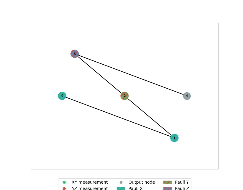
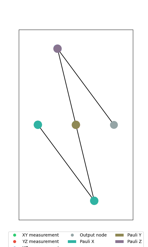
Pauli measurement demo graph:
Input nodes: [0]
Output nodes: [4]
Pauli measurement nodes (will show bordered patterns):
  - X measurement (θ=0°): Green center + Blue border (XY+XZ planes)
  - Y measurement (θ=90°): Red center + Green border (YZ+XY planes)
  - Z measurement (θ=180°): Blue center + Red border (XZ+YZ planes)
Individual nodes:
  Node 0: XY plane, angle=0.000 (0.0°)
  Node 1: XY plane, angle=0.000 (0.0°)
  Node 2: YZ plane, angle=1.571 (90.0°)
  Node 3: XZ plane, angle=3.142 (180.0°)
Displayed Pauli demo graph

--- Larger nodes without labels ---
Displayed Pauli demo graph without labels

--- Without legend to avoid overlap ---
Displayed Pauli demo graph without legend