Non-Unitary Parity Projection in MBQC

A 3-node star graph implements the Kraus branch

\[K_s = \frac{I + (-1)^s\, Z_0 Z_1}{2}\]

on the two data qubits when the central ancilla is measured in the \(X\) basis. Starting from \(|{+}{+}\rangle\), the two branches produce Bell states:

\[\begin{split}s = 0 &\;\longrightarrow\; |\Phi^+\rangle = \frac{|00\rangle + |11\rangle}{\sqrt{2}} \\ s = 1 &\;\longrightarrow\; |\Psi^+\rangle = \frac{|01\rangle + |10\rangle}{\sqrt{2}}\end{split}\]

This demonstrates measurement-induced entanglement: a genuinely non-unitary operation realised by a single MBQC measurement.

import matplotlib.pyplot as plt
import numpy as np

from graphqomb.common import Axis, AxisMeasBasis, MeasBasis, Sign
from graphqomb.graphstate import GraphState
from graphqomb.pattern import print_pattern
from graphqomb.qompiler import qompile
from graphqomb.simulator import PatternSimulator, SimulatorBackend
from graphqomb.visualizer import visualize

Build the star graph: two data qubits connected to one ancilla.

nodes = ["q0", "q1", "anc"]
edges = [("q0", "anc"), ("q1", "anc")]
inputs = ["q0", "q1"]
outputs = ["q0", "q1"]

meas_bases: dict[str, MeasBasis] = {
    "anc": AxisMeasBasis(Axis.X, Sign.PLUS),
}

graph, node_map = GraphState.from_graph(
    nodes=nodes,
    edges=edges,
    inputs=inputs,
    outputs=outputs,
    meas_bases=meas_bases,
    coordinates={"q0": (0.0, 0.0), "q1": (2.0, 0.0), "anc": (1.0, 1.0)},
)

# No corrective feedforward: keep the genuine non-unitary branch.
xflow: dict[int, set[int]] = {}

pattern = qompile(graph, xflow)
print("pattern depth        :", pattern.depth)
print("pattern max space    :", pattern.max_space)
print("pattern active volume:", pattern.active_volume)
print_pattern(pattern)

pattern depth        : 2
pattern max space    : 3
pattern active volume: 7
N: node=2, coord=(1.0, 1.0)
E: nodes=(0, 2)
E: nodes=(1, 2)
TICK
M: node=2, plane=Plane.XY, angle=0
TICK
X: node=0
Z: node=0
X: node=1
Z: node=1
0 more commands truncated. Change lim argument of print_pattern() to show more

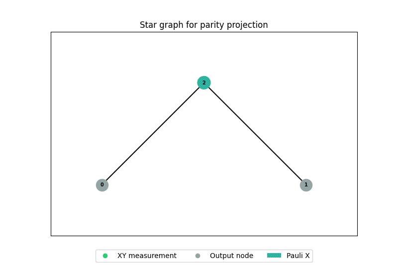
Visualize the star graph.

ax = visualize(graph, show_node_labels=True)
ax.set_title("Star graph for parity projection")
plt.show()

Reference Bell states for verification.

PHI_PLUS = np.array([1, 0, 0, 1], dtype=complex) / np.sqrt(2)
PSI_PLUS = np.array([0, 1, 1, 0], dtype=complex) / np.sqrt(2)

anc_node = node_map["anc"]


def run(seed: int) -> None:
    """Run the pattern once and report which Bell state appears."""
    sim = PatternSimulator(pattern, SimulatorBackend.StateVector)
    sim.simulate(rng=np.random.default_rng(seed))

    out = sim.state.state().ravel()

    overlap_phi = abs(np.vdot(PHI_PLUS, out))
    overlap_psi = abs(np.vdot(PSI_PLUS, out))

    s = int(sim.results[anc_node])
    print(f"seed={seed}, ancilla result s={s}")
    print(f"  |<Phi+|out>| = {overlap_phi:.6f}")
    print(f"  |<Psi+|out>| = {overlap_psi:.6f}")
    print()


# These two seeds give the two different branches with NumPy's default_rng.
run(seed=0)
run(seed=2)

seed=0, ancilla result s=0
  |<Phi+|out>| = 1.000000
  |<Psi+|out>| = 0.000000

seed=2, ancilla result s=1
  |<Phi+|out>| = 0.000000
  |<Psi+|out>| = 1.000000